Distributed Control Systems – An Evolution

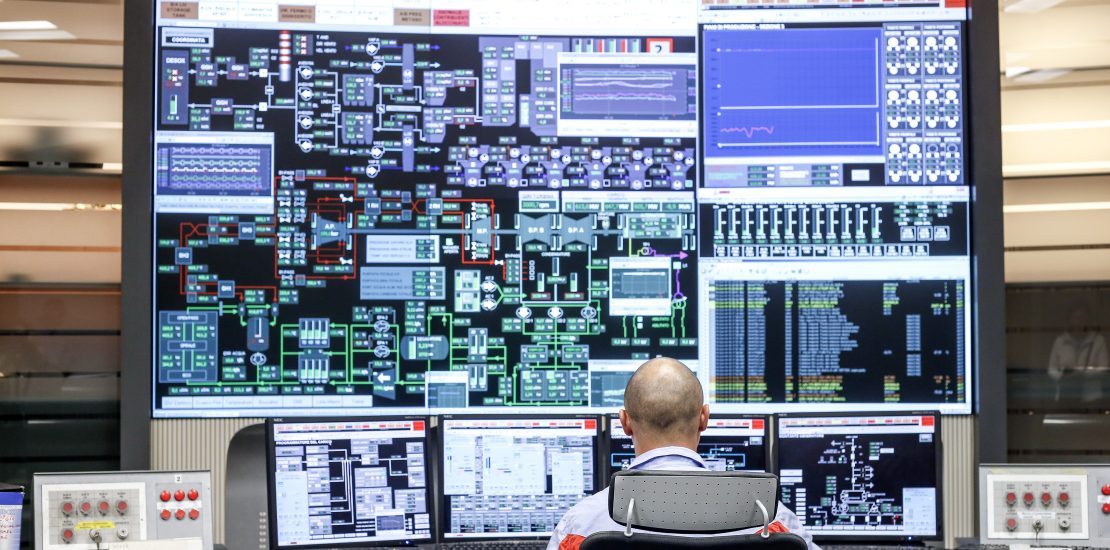
Today’s automation system or process control system, like virtually everything these days, is built from an array of special purpose microprocessors along with computers and networked servers. These systems are referred to as “DCS” systems, which translates to “Distributed Control System”.

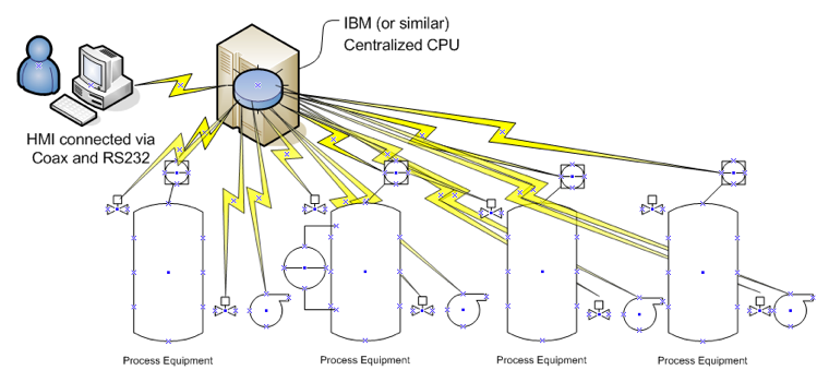
Many years ago, there were big computers that were centralized, with thousands of wires going to and from them. All the program logic was centrally located within each of these large computers. These general-purpose computers did many things, from payroll and accounting to databases, so perhaps it seemed sensible to have them perform industrial automation as well.

An industrial control system servicing a big factory might be connected to several thousand sensors and actuators. This meant the costly situation of several thousand wires running up to several hundred miles. Figure 1 illustrates the congestion associated with just a few pieces of process equipment.

In the 1980s, a new approach emerged, which was a coordinated network of computers, distributed much closer to the equipment. This “Distributed” approach became very popular due to numerous advantages. For automation systems, the term “Distributed Control Systems” became ubiquitous in our industry. Other terms that are often used are “Process Control System,” “Process Automation System” or “Industrial Control System”, but none have gained common acceptance like “DCS”.

There is a wide variation between these categories. As technology advanced, so did control systems, evolving to incorporate a more distributed architecture, and a plethora of networks to support this distribution. This generally follows a ”client-server” architecture, such that most logic and control execution is performed at localized devices called controllers.

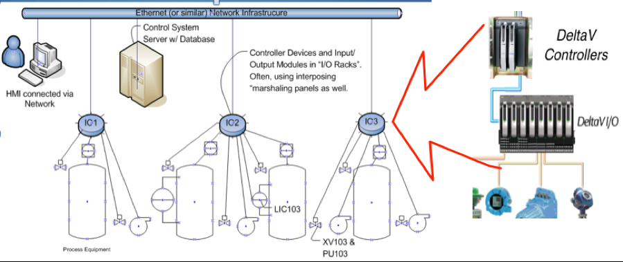
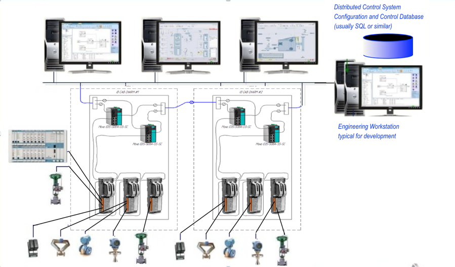
In typical modern DCS systems, controllers are mounted in chassis racks, along with appropriate interface modules to process the field device signals. These racks are located closer to the process equipment, thus reducing the length of the hundreds of field device signal cables. Process data is consolidated into the controller for control functions and reporting over the network to the HMI and operator display graphics. There still is a central server, but its role is greatly diminished, relegated to being a central location for the system-wide database, used only to download into the controllers as needed, and for administrative functions. Figure 2 illustrates this typical DCS setup.

Figure 3 shows the architecture of an earlier phase in the development of the Distributed Control System, which we will refer to as “DCS version 1.0”. In this diagram illustrating “DCS version 1.0” there is physical and logical grouping within each control and I/O rack, so there needs to be thought about signal and I/O rack physical locations during the design phase of an installation.

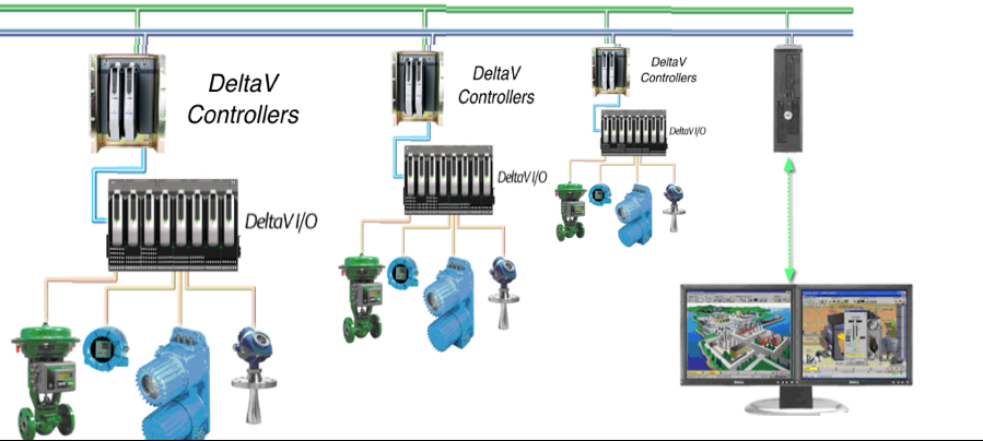
In Figure 4, we see the evolution to “DCS version 2.0”, which is specifically an illustration of an Emerson DeltaV system. This highlights developments that have been responsible for new, cost effective advancements in control systems. The signal processing and control calculation, logic and even sequencing is distributed, downloaded into completely autonomous controllers – controllers vastly more powerful than previous generation DCS systems possessed.

Another common industry term is “PLC”, which stands for “Programmable Logic Controller”, again due to historical usage. In the modern context, the principal distinction between PLC and DCS controllers is that the PLC’s programming language is more visualized in sometimes complex relay connections, using the software equivalent of wires and open or closed contacts, referred to as “Ladder Logic”, while DCS system configuration is a more multi-faceted database and mathematical calculation driven, relying on functions with inputs and outputs wired together.

PLC systems are better suited to machinery control, especially servo motors, conveyors and robot systems due to their logic oriented structure, while DCS systems are better suited performing more elaborate process control and optimization, especially batch recipe management and sequencing. It should be said that either system can certainly manage any of theses functions, but it’s a question of which is best suited for which role. It is a question of time and effort to achieve the desired functionality.

When a technology is considered for a task, any kind of technology, the ease of use, ease of deployment and ease of maintenance all must be taken into account. An electrician working on a motor that won’t start will have much greater ease of use, and hence quicker results by looking at open or closed contacts, highlighted with their active status, than reading boolean expression consisting of “AND” and “OR” or “NAND” gates.

Manufacturers tend to be aligned with one or the other of these two control types (DCS vs. PLC), with the familiar names like: Emerson DeltaV, Honeywell Experion, ABB 800xA, Foxboro Invensys and Siemens PCS7 (now PCS Neo) being categorized as “DCS”. Rockwell Allen Bradley, Siemens (Step 7 family), Schneider Modicon, Omeron, Opto and Phoenix are representative of systems categorized as “PLC”s.  These are arbitrary distinctions in that these categorizations are more historical, since the automation systems of today quickly blur these boundaries with considerable overlap.

A most striking example of this is Emerson’s most recent development, the “PK” generation of controller which draws upon the sophistication, and network integration, and ease of use it inherits from the DCS environment, while simultaneously drawing in the autonomous nature and scalability (start small, grow big). An apparent goal, well achieved, was the almost native integration with other vendors PLC equipment, a very common circumstance with skid vendors who build their complete systems on PLC systems.  This is most often Rockwell, Siemens or Schneider, but other OEM vendors as well.

The easier an integration effort is to incorporate these systems into the larger plant automation architecture, the more quickly a project is successful. It would bare pointing out that Emerson “PK” controllers is but one solution of overall plant integration, since there also are other popular solutions from other vendors, notably Rockwell sophisticated FactoryTalk and PlantPAx products.

It should be pointed out that while DCS vendors have started offering scalable, downward compatible solutions to be competitive with PLCs, the PLC vendors have conversely been expanding their products upward, to embrace a more advanced features and sophistication to be quite competitive with systems from the DCS vendors.

A significant development within industrial control systems is that of “Electronic Marshaling”. Traditionally, marshaling referred to the field cabling signal data coming from the I/O devices being connected to marshaling termination strips as it enters the I/O cabinets. Then the signals data is connected via jumper wiring to the termination of the appropriate I/O modules. The physical location of the I/O modules within particular chassis automatically associate that module’s signals with the controller located within that chassis.

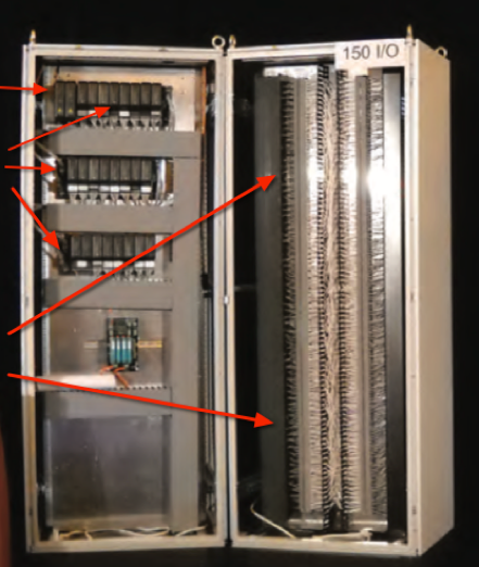
Figure 5 shows this traditional marshaling termination used in a DCS version 1.0 system. On the top left position, we see two controllers (redundant) for the chassis/racks. There are three chassis populated with I/O modules. The modules can process input or output signal types or either analog or discrete devices, as well as pulse counting, and thermocouple or RTDs.

The entire right hand side of this panel is occupied by the marshaling termination for 150 I/O signals. We see the field wiring cables coming in from the right hand side, then cable harness (hidden by the Panduit covers) transiting from there to the I/O modules on the left side.

In the era of DCS version 2.0, “Electronic Marshaling” is not exactly new, having begun with the introduction of CHARMS I/O almost a decade ago. Such innovations, while compelling, often only make sense in new system implementations.

The electronic marshaling concept makes use of single channel, individual field devices, signal conditioning, digitizing, and termination all in one module, named “CHARMS”, for “CHARacterization ModuleS”.

In DCS 1.0 designs, a module contains the scaling and digitizing electronics to convert 8 or 16 channels of analog readings into digitally encoded words on a network. This conversion is performed on the individual channels, giving ultimate flexibility to mix and match signal types, and simplify ad-hoc changes.

This enhanced design allows for eliminating marshaling panels, increasing density within cabinets, simplifying engineering and accommodating I/O changes dynamically, and conveniently during installation and commissioning. As if this wasn’t enough, the CHARMS are “hot swappable”, meaning a failure can be addressed with a “pluck and replace” of an offending module without the slightest interruption of adjacent signal processing. This contrasts to older systems where a module replacement meant powering down of an entire chassis, or at minimum, of all the channels on a multi-channel module.

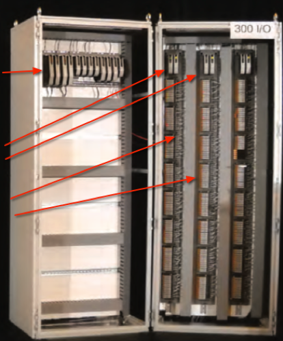
What does this DCS 2.0, with its Electronic Marshaling, look like? Figure 6 depicts a DCS 2.0 I/O rack with CHARMS modules. It is much more consolidated and organized. There are still the controllers and communications support, but the chassis, full of I/O modules are gone.  Likewise, blocks of single channel signal processors, called CHARMS modules, have replaced the terminal strips, previously used for marshalling. 

Each column of these CHARMS modules (up to 96 modules) is serviced by network communications modules and are now accessible network-wide, not limited to the local chassis and controller.  This enhanced use of space now supports 300 I/O device signals, twice which was previously supported.

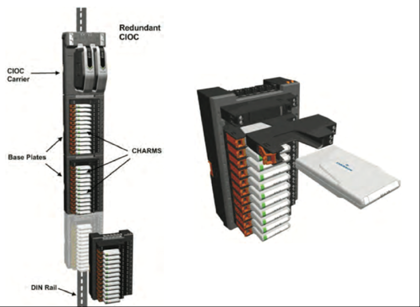
Figure 7 illustrates how the Individual modules are inserted into a base carrier and connected together to communicate to the communication processors “CIOC” (short for “CHARMS I/O Communications”).

Using this approach, significant savings are realized in engineering design, drawings, wiring, and commissioning costs. The elimination of terminal strips, jumper wiring, simplified wiring termination diagrams, and reduced termination and commissioning times realize considerable cost savings. When considering a 5-10 minute installation time per termination point, including checkout & commissioning, the savings can be 350-700 hours for a 1,000 I/O sized system. This also results in fewer points to get “lost” or mislabeled, since every wire in a cabinet requires (or should have) a wire label on each end. Fewer errors mean faster startups with higher confidence and lower risk.

It’s easy to see why customers are embracing this new innovation. That outlines the history of DCS systems, but what’s next to come? The evolution is ongoing, and admittedly not limited to one vendor. However, there is certainly a lot of innovation emerging in the developments highlighted in this discussion.

Written By

John Andrews
Director of Automation